2018-06-11
This post describes atmospheric scattering model that was implemented in Appear by Jetlag 4k intro, party version of which took 12th place in 4k intro compo at Revision 2018 demoparty.
(In case you're not familiar with demoscene and demoparties, 4k intro is an executable file limited to 4096 bytes that is supposed to render complex music and visuals in real-time for a few minutes to awe the audience ("how is this even possible?! my empty Unity Engine build is more than 50 megabytes!"). There are competitions for these things that take place at various demoparties, mainly across the Europe.)
Before we begin, you can watch the final version of the intro on youtube. Or, better, you can download the binary and run it on your Windows PC (beware, fast GPU is required).
Music for the intro is made by keen using 4klang softsynth. Code and visuals were made by me.
Here I won't describe other parts of the intro, e.g. city geometry or our tooling. You can check out complete source code for the intro if you feel brave enough.
This intro was born out of desire to make something really quick for Revision. Somewhere mid-March we realized that we don't have enough resources to do a proper 4k entry, so it had to be something simple that we could make in a few evenings. Doing yet another raymarching thing seemed boring, so there had to be something else in it too.
The idea that we chose to stick with was some kind of raymarched landscape lit with atmospheric scattering. Scattering looks rather cool, while being simple to implement and relatively compact to fit within 4 kilobytes. The fact that it's ridiculously slow could be masked by making slow-paced scenes paired with ambient music. Rendering artifacts due to low integration steps count could be mitigated by adding noise to integration sample steps (kind of monte-carlo method). Denoizing could be done by blending consecutive frames, because they wouldn't change very much, due to ambient nature of the intro.
While keen had made the music for the intro a couple of weeks before the party, I haven't really started working on it until I was on a plane to Germany for the party (I fell sick with a very bad flu and was essentially incapacitated for two weeks before the party; I was barely able to start recovering before the scheduled flight), going through scattering equations and coding a model prototype during the flight. We ended up hastily hacking together the party version at the party place during only a few hours before the deadline (while I was sleep-deprived, recovering from the flu, and also being constantly interrupted by participating in Shader showdown livecoding compo I hope this explains much).
The party version had only rudimentary city geometry, and also had a lot of scattering artifacts and noise.
The final version was made much later, mostly live (mostly in Russian).
(Disclaimer: I am not a graphics programmer professionally, so please bear with me if I mislabel or misunderstand anything. Please correct me if you see something wrong!)
Scattering model was essentially borrowed from "High Performance Outdoor Light Scattering Using Epipolar Sampling" article by Egor Yusov, published in GPU Pro 5, with epipolar thing completely disregarded.
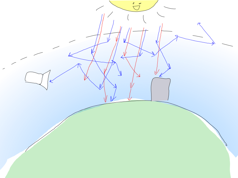
Photons coming from the sun enter Earth's atmosphere and interact with air particles. A photon can be scattered by particle, which means just changing its direction. Or it can be absorbed, which means that the photon is lost and its energy is transformed into some other form. Both processes are probabilistic and depend on photon's energy, which is more or less equivalent to its percieved color. "Red" photons have lower probability of interacting with the atmosphere, so they mostly get through intact. The "blue" ones, however, are quite more likely to be scattered, so they change direction a lot and may travel far from original entry point before finally getting through to an observer.

These photon-air interactions can be described in terms of
\(\beta^s(x)\), amount of light scattered per unit length at point \(x\)
\(\beta^a(x)\), amount of light absorbed per unit length at point \(x\)
\(\beta^e(x) = \beta^s(x) + \beta^a(x)\), total amount of light lost per unit length at point \(x\)
phase function \(p(\alpha)\), angular distribution of the scattered light, meaning amount of light that will be scattered from incident ray towards outgoing ray, where \(\alpha\) is the angle between these rays
Air is modelled as a mix of two types of particles: molecules and aerosols. These are described by Rayleigh and Mie theories respectively, and have different \(\beta\) and \(p(\alpha)\) parameters.
For both models we assume that air density decreases exponentially with height: \(\rho = \rho_0e^{-\frac{h}{H}}\), where \(\rho_0\) is density at sea level. Scattering coefficients \(\beta\) are proportional to air density \(\rho\), and their values given below are for sea level.
\(p_R(\alpha) = \frac{3}{16\pi}(1+\cos^2(\alpha))\) [Nishita et al. 93, Preetham et al. 99]
\(\beta_R^a = 0\)
\(\mathbf{\beta_R^e} = \mathbf{\beta_R^s} = (5.8, 13.5, 33.1)_{rgb}10^{-6}m^{-1}\) [Riley et al. 04, Bruneton and Neyret 08]
\(H_R = 7994m\) [Nishita et al. 93]
\(p_M(\alpha) = \frac{1}{4\pi}\frac{3(1-g^2)}{2(2+g^2)}\frac{1+\cos^2(\alpha)}{(1 + g^2 - 2g\cos(\alpha))^\frac{3}{2}}\) [Nisita et al. 93, Riley et al. 04], where \(g = 0.76\) [Bruneton and Neyret 08]
\(\beta_M^s = 2\cdot10^{-5}m^{-1}\) [Bruneton and Neyret 08]
\(\beta_M^e = 1.1\beta_M^s\)
\(H_M = 1200m\) [Nishita et al. 93]
Notice that Mie scattering is color-independent, and also mostly happens only in lower layers of atmosphere.
We approximate the scattering process by casting a ray per camera pixel and calculating how much light is incoming from this ray direction. Each ray corresponds to three colors, as if there are three photons, with R-, G- and B-colored energies, that are flying together.
Incoming light that should be registered by camera pixel can be calculated by factoring in the following processes:
In-scattering. Light coming from the sun is in-scattered to fly in camera direction.
Absorbtion. Light already travelling along the ray is lost by being absorbed by air.
Scattering. Light already travelling along the ray is lost by being scattered away by air.
Only single source of in-scattering is supported, which is the sun. We assume that multiple scattering is relatively infinitesimal (this is not true for e.g. twilight, but oh well).
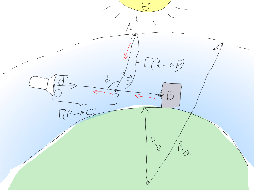
This setup is illustrated in the following picture:

Amount of light that should be registered at camera pixel point \(O\) can be calculated as \(\mathbf{L} = \mathbf{L_{in}} + \mathbf{L_{BO}}\), where \(\mathbf{L_{in}}\) is light in-scattered from the sun, and \(\mathbf{L_{BO}}\) is amount of light from object point \(B\) reaching \(O\).
\(\mathbf{L_{BO}} = \mathbf{L_O} e ^ {-\mathbf{T}(B \rightarrow O)}\), where \(\mathbf{L_O}\) is amount of light emitted at point \(B\) in camera direction.
\(\mathbf{T}(B \rightarrow O)\) is called optical depth along the path from \(B\) to \(O\) and can be calculated as:
\(\mathbf{T}(B \rightarrow O) = \int_B^O(\beta_M^e(s) + \mathbf{\beta_R^e}(s))ds\)
Noticing that \(\beta\)s consist of sea-level constants and variable density, we can write it down as:
\(\mathbf{T}(B \rightarrow O) = \beta_M^e \cdot \int_C^D \rho_M(s) ds + \mathbf{\beta_R^e} \int_C^D \rho_R(s) ds\)
I intentionally don't expand \(\rho\) functions here, because that's how we'll compute them below. Note that \(\beta\) are constant vectors (at least \(\mathbf{\beta_R}\) is, but \(\beta_M\) must also be for consistency). \(\rho\)-parts under integrals are scalar.
To calculate in-scattered sunlight \(\mathbf{L_{in}}\), we need to integrate all in-scattered light coming from the sun for all points \(P\) along the \(OB\) and attenuate it with \(\mathbf{T}(P \rightarrow O)\).
Light reaching point \(P\) from the sun can be written down as \(\mathbf{L_P} = \mathbf{L_{sun}}e^{-T(A \rightarrow P)}\), where \(\mathbf{L_{sun}}\) is sun intensity and \(A\) is the point where sun direction ray \(\vec{s}\) from point \(P\) reaches atmosphere top. The portion of this light that will be scattered in camera direction is \(\mathbf{L_P} \cdot (\mathbf{\beta_R^s}(s)p_R(\alpha) + \beta_M^s(s) p_M(\alpha))\), and after that it will also have to go through \(P \rightarrow O\) amount of air. This gives:
\(\mathbf{L_{in}} = \int_B^O \mathbf{L_P}(s) \cdot (\beta_M^s(s) p_M(\alpha) + \mathbf{\beta_R^s}(s)p_R(\alpha)) \cdot e ^ {-\mathbf{T}(P(s) \rightarrow O)} ds\)
We can simplify this integral by noticing that:
\(\alpha\) is constant per camera pixel ray (sun is really far away, so rays of light coming from it are effectively parallel)
\(\beta\) scattering coefficients are sea-level constants multiplied by density functions
\(p(\alpha)\) phase functions have common multipliers
Grouping similar things together, we get:
\(\mathbf{L_{in}} = \mathbf{L_{sun}} (1+\cos^2(\alpha)) (\frac{\frac{1}{4\pi}\frac{3(1-g^2)}{2(2+g^2)}}{(1 + g^2 - 2g\cos(\alpha))^\frac{3}{2}}\beta_M^s \cdot \mathbf{I_M} + \frac{3}{16\pi} \mathbf{\beta_R^s} \cdot \mathbf{I_R})\), where
\(\mathbf{I_M} = \int_B^O \rho_M(s) e^{-\mathbf{T}(A \rightarrow P(s)) - \mathbf{T}(P(s) \rightarrow O)} ds\), and
\(\mathbf{I_R} = \int_B^O \rho_R(s) e^{-\mathbf{T}(A \rightarrow P(s)) - \mathbf{T}(P(s) \rightarrow O)} ds\)
These integrals differ only by density terms, and their exponential parts are the same (which is convenient).
They also cannot be computed analytically. So we're gonna compute them numerically (as the original papers advises against!) by raymarching!
We will do the dumbest and naivest thing possible: \(\int_A^B f(x) dx \approx \frac{\left |B - A \right |}{N} \sum_{i=0}^N f(A + i \cdot \frac{\vec{B - A}}{N})\)
We will raymarch in the direction opposite to the light direction: from camera \(O\) to object \(B\). \(O \rightarrow B\) will be divided into \(N\) steps.
First, we'll zero-initialize variables :
vec2 (for separate Mie and Rayleigh terms) total accumulated depth \(\mathbf{T}(P(s) \rightarrow O)\)
vec3 (RGB) \(\mathbf{I_M}\), \(\mathbf{I_R}\)
For each march step \(P_i\) between \(O\) and \(B\) we will:
Cast a ray in sun direction \(\vec{s}\) and get the point of its intersection with atmosphere top \(A_i\)
Compute \(\mathbf{T}(A \rightarrow P_i)\) by first computing \(\int_A^{P_i}\rho_M(s)ds\) and \(\int_A^{P_i}\rho_R(s)ds\) with similar raymarching process (with M steps) and then multiplying them by corresponding \(\beta_M^e\) and \(\mathbf{\beta_R^e}\) constants
Compute \(\mathbf{T}(P_i \rightarrow O)\) by just adding \(\rho_i(s) \cdot ds\) to its value from previous \(P_i\)
Accumulate \(\mathbf{I_R}\) and \(\mathbf{I_M}\) using these values
After raymarching is done, the final color will be calculated by
Calculating \(\mathbf{L_{BO}}\) term using accumulated \(\mathbf{T}(P_i \rightarrow O)\): with \(P_i\) reaching \(B\) it became \(\mathbf{T}(B \rightarrow O)\)
Multiplying \(\mathbf{I_R}\) and \(\mathbf{I_M}\) with corresponding constants, adding them together and getting \(\mathbf{L_{in}}\)
Adding \(\mathbf{L_{in}}\) and \(\mathbf{L_{BO}}\) together
Here is a simplified and commented source taken (almost) directly from the intro itself.
const float R0 = 6360e3; // Earth surface radius
const float Ra = 6380e3; // Earth atmosphere top raduis
const vec3 bR = vec3(58e-7, 135e-7, 331e-7); // Rayleigh scattering coefficient
const vec3 bMs = vec3(2e-5); // Mie scattering coefficients
const vec3 bMe = bMs * 1.1;
const float I = 10.; // Sun intensity
const vec3 C = vec3(0., -R0, 0.); // Earth center point

// Calculate densities $\rho$.
// Returns vec2(rho_rayleigh, rho_mie)
// Note that intro version is more complicated and adds clouds by abusing Mie scattering density.
// That's why it's a separate function
vec2 densitiesRM(vec3 p) {
    float h = max(0., length(p - C) - R0); // calculate height from Earth surface
    return vec2(exp(-h/8e3), exp(-h/12e2));
}

// Basically a ray-sphere intersection. Find distance to where rays escapes a sphere with given radius.
// Used to calculate length at which ray escapes atmosphere
float escape(vec3 p, vec3 d, float R) {
    vec3 v = p - C;
    float b = dot(v, d);
    float det = b * b - dot(v, v) + R*R;
    if (det < 0.) return -1.;
    det = sqrt(det);
    float t1 = -b - det, t2 = -b + det;
    return (t1 >= 0.) ? t1 : t2;
}

// Calculate density integral for optical depth for ray starting at point `p` in direction `d` for length `L`
// Perform `steps` steps of integration
// Returns vec2(depth_int_rayleigh, depth_int_mie)
vec2 scatterDepthInt(vec3 o, vec3 d, float L, float steps) {
    // Accumulator
    vec2 depthRMs = vec2(0.);

    // Set L to be step distance and pre-multiply d with it
    L /= steps; d *= L;

    // Go from point P to A
    for (float i = 0.; i < steps; ++i)
        // Simply accumulate densities
        depthRMs += densitiesRM(o + d * i);

    return depthRMs * L;
}


// Global variables, needed for size
vec2 totalDepthRM;
vec3 I_R, I_M;

vec3 sundir;

// Calculate in-scattering for ray starting at point `o` in direction `d` for length `L`
// Perform `steps` steps of integration
void scatterIn(vec3 o, vec3 d, float L, float steps) {

    // Set L to be step distance and pre-multiply d with it
    L /= steps; d *= L;

    // Go from point O to B
    for (float i = 0.; i < steps; ++i) {

        // Calculate position of point P_i
        vec3 p = o + d * i;

        // Calculate densities
        vec2 dRM = densitiesRM(p) * L;

        // Accumulate T(P_i -> O) with the new P_i
        totalDepthRM += dRM;

        // Calculate sum of optical depths. totalDepthRM is T(P_i -> O)
        // scatterDepthInt calculates integral part for T(A -> P_i)
        // So depthRMSum becomes sum of both optical depths
        vec2 depthRMsum = totalDepthRM + scatterDepthInt(p, sundir, escape(p, sundir, Ra), 4.);

        // Calculate e^(T(A -> P_i) + T(P_i -> O)
        vec3 A = exp(-bR * depthRMsum.x - bMe * depthRMsum.y);

        // Accumulate I_R and I_M
        I_R += A * dRM.x;
        I_M += A * dRM.y;
    }
}

// Final scattering function
// O = o -- starting point
// B = o + d * L -- end point
// Lo -- end point color to calculate extinction for
vec3 scatter(vec3 o, vec3 d, float L, vec3 Lo) {

    // Zero T(P -> O) accumulator
    totalDepthRM = vec2(0.);

    // Zero I_M and I_R
    I_R = I_M = vec3(0.);

    // Compute T(P -> O) and I_M and I_R
    scatterIn(o, d, L, 16.);

    // mu = cos(alpha)
    float mu = dot(d, sundir);

    // Calculate Lo extinction
    return Lo * exp(-bR * totalDepthRM.x - bMe * totalDepthRM.y)

    // Add in-scattering
        + I * (1. + mu * mu) * (
            I_R * bR * .0597 +
            I_M * bMs * .0196 / pow(1.58 - 1.52 * mu, 1.5));
}It's cool, but nothing that couldn't have been faked by some clever gradients.
Clouds with god rays are harder to fake, so lets add them.
Idea is to assume that clouds can be approximated aerosols and add some noise to the Mie coefficient at higher altitudes. This may be not physically correct, and I have no idea how clouds are really approximated in computer graphics (I do have a few papers in reading queue, but I certainly couldn't access them when I prototyped this in mid-air).
With that in mind, densitiesRM function becomes:
const float low = 1e3, hi = 25e2;

// vec4 noise24(vec2 v) just reads from noise texture
// float t is time

float noise31(vec3 v) {
    return (noise24(v.xz).x + noise24(v.yx).y) * .5;
}

vec2 densitiesRM(vec3 p) {
    float h = max(0., length(p - C) - R0);
    vec2 retRM = vec2(exp(-h/8e3), exp(-h/12e2) * 8.);

    // Clouds are between 1km and 2.5km
    if (low < h && h < hi) {
        vec3 v = 15e-4 * (p + t * vec3(-90., 0., 80.));

        // All of this is <s>carefully</s> randomly tweaked to look okay'ish for the intro
        retRM.y +=
            250. *
            step(v.z, 38.) *
            smoothstep(low, low + 1e2, h) *
            smoothstep(hi, hi - 1e3, h) *
            smoothstep(.5, .55, // core part: fractal value noise
                .75 * noise31(v)
                + .125 * noise31(v*4. + t)
                + .0625 * noise31(v*9.)
                + .0625 * noise31(v*17.)-.1
            );
    }

    return retRM;
}
At this point atmosphere starts to have too many artifacts due to low sampling count (our \(N\) and \(M\) raymarch steps). Universally increasing this count is not feasible: it becomes too slow really fast, and many artifacts, especially in the horizon, are still visible.
Solutions hacks that I came up with:
Mask horizon by adding "mountains" raymarched geometry
Limit clouds to area around camera (distant clouds are glitchy)
Add slight random offset for each ray: for (float i = pixel_random.w; i < steps; ++i) { This adds visible noise, which is mostly temporally-filtered by blending with the previous frame.
Increase integration sampling count for areas prone to artifacts due to high details (e.g. cloud layers). This explains this weird function separation you might have noticed above.
// inside scatterIn() function loop
    vec2 depthRMsum = totalDepthRM;
    float l = max(0., escape(p, sundir, R0 + hi));
    if (l > 0.) // Do 16 steps below clouds top
        depthRMsum += scatterDepthInt(p, sundir, l, 16.);
    // do only 4 steps above
    depthRMsum += scatterDepthInt(p + sundir * l, sundir, escape(p, sundir, Ra), 4.);
// inside scatter() function
// nearest 10km get more steps
float l = 10e3;
if (L < l)
scatterIn(o, d, L, 16.);
else {
scatterIn(o, d, l, 32.);
// Only 8 steps if farther than 10km
scatterIn(o+d*l, d, L-l, 8.);
}Now that the atmosphere ready, it's time to combine it with scene geometry.
It's straightforward to do: just come up with pixel color using e.g. traditional distance fields raymarching, and pass it as Lo argument into scatter() function, and L set to distance ray travelled. If ray has escaped, then L should be calculated by escape() function, and Lo is set to zero.
That's it.
... No, that's not really it. It does require quite a bit of tweaking to look convincing. I'm afraid I can't really give any good advice here.
After being processed by shader minifier the final scattering code that goes into intro is at about 1500 bytes. Crinkler brings it down to about 700 bytes, which is roughly 30% of all shader code.
I am not good at computer graphics.